Flip/Vellum/MPM Lecture - VFX319

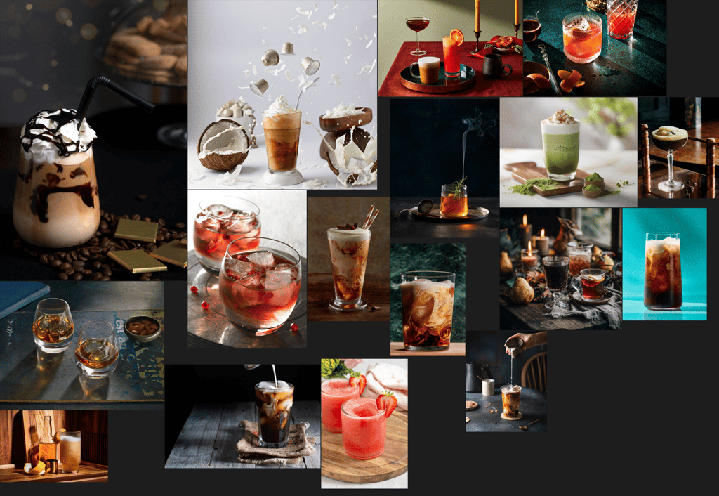
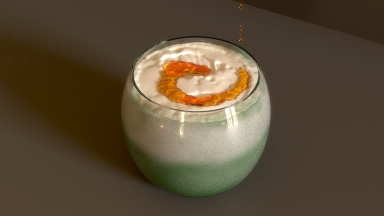
Render Test

Reference

Overview:

• Introduction to FLIP, Vellum Fluid, and MPM - basic concepts and setup

• Mixing colors between two fluids

• Icy fractured look inside an ice cube

• Handy Houdini tips

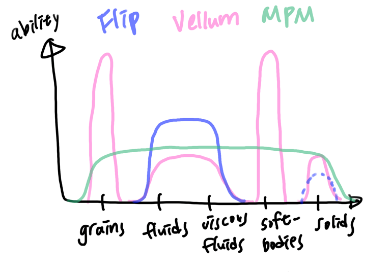
Material Simulation Strengths: FLIP, Vellum Fluid, and MPM

FLIP Fluids

• Type: Hybrid Particle-Grid

  • Effect of Type:

    Uses particles for mass and a grid for velocity/pressure

    accurate for real fluid physics, especially with large volumes and complex flows

• Best Use: Rivers, oceans

Vellum Fluids(H19)

• Type: Position-Based Dynamics

  (not volume-based)

  • Effect of Type:

    Works by moving points to satisfy constraints

    fast and stable, not super realistic for heavy fluids

• Best Use: Small fluid splashes, light water, soft bodies

MPM(H20)

• Type: Material Point Method (particles + grid)

  • Effect of Type:

    Tracks particles for the material, but computes forces on a grid

    Works for solids, snow, soil, clay, and fluids interacting with solids

    Can handle chunky, heavy, or materials that bend, break, or compress

• Best Use: Snow, mud, mixing solids and fluids

Source:

• https://www.sidefx.com/docs/houdini/nodes/sop/flipsolver.html

• https://www.sidefx.com/docs/houdini/vellum/fluidsetups.html

• https://www.sidefx.com/docs/houdini//nodes/sop/mpmsolver.html

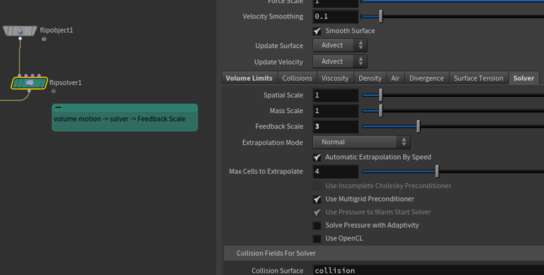
Flip solver

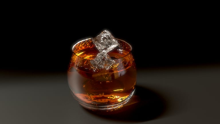
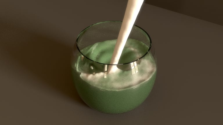
For this project, I plan to experiment with two simulations: one showing an ice cube dropping into a glass of whiskey, and another creating a matcha latte with four different components: matcha, milk, cream, and honey.

To begin, it’s essential to understand the basic concepts of the three solvers I’ll be using: FLIP, Vellum Fluid, and MPM, as shown above. I first tested the FLIP solver for the simulation, but since FLIP is mainly designed for large-scale fluid simulations, the ice cube sank to the bottom of the cup instead of floating.

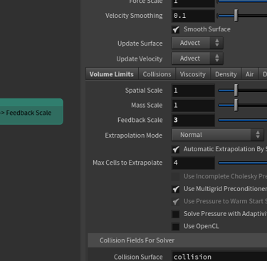
In the FLIP Solver, under Volume Motion -> Solver -> Feedback Scale, the default value is set to 0. You can experiment by increasing it to 1 or 2 to create more interaction between the fluid and the solid object. However, even with these adjustments, the simulation still didn’t perform as expected, primarily due to its small scale. When using an ocean source, the FLIP solver can accurately keep objects floating on the surface, but at smaller scales, this behavior becomes less reliable.

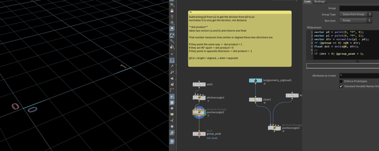
Dot product

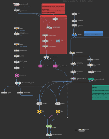
For the FLIP simulation, my cup collider is very thin, which can cause volume loss during the simulation. To fix this, I needed to make the cup thicker, but I only wanted to extrude the outside faces, keeping the inside faces unchanged.

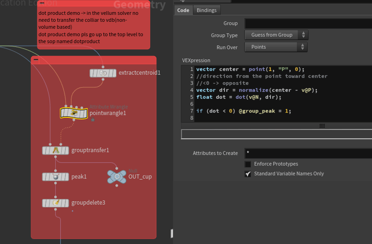
Instead of manually selecting all the outside faces one by one, I used a dot product method to identify the points facing away from the cup’s center. This allows you to select and extrude only the outer faces automatically.

I placed a point at the center of the cup and subtracted the center position from each point (@P) to get the direction from the center to every point. I then normalized this vector to focus only on direction, ignoring distance.

Next, I used the dot product between this direction vector and each point’s normal. If the dot product indicates that the point’s normal is pointing opposite the center, I added it to a group called “peak”.

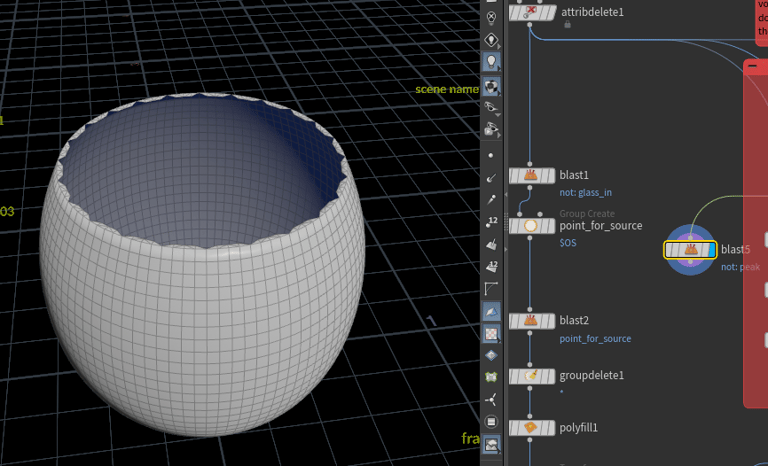
when it extruded, the inside faces move

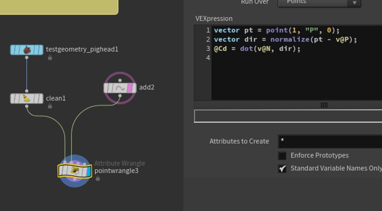
two points demo

@Cd demo

Vellum Fluid

Next, I chose to use the Vellum Solver to simulate the interaction between the ice cube and the fluid. You can see the basic setup for the Vellum fluid simulation here.

First, you need a Vellum source geometry connected to the solver, along with constraints and collision geometry. In the Vellum Constraints setup, set the type to Fluid. This allows you to adjust key parameters such as particle size, density, and viscosity for the fluid. Before feeding it into the solver, I added an @v attribute to the source so that I could control its velocity directly within the simulation.

For the ice cube, I used a Tet Conform node followed by Vellum Constraints, setting the type to Tetrahedral Stretch to make it behave more like a solid. Here, you can control its density, stiffness, and damping values.

Understanding how stiffness and damping work is very important:

Damping:

• 0 -> no damping -> tets can move and bounce freely (soft or jelly-like)

• 1 -> critically damped -> no bouncing, stops immediately when stretched

• Stiffness -> determines how strongly the constraint resists stretching

• Damping -> controls how quickly the constraint loses energy and stops moving

By balancing these two parameters, you can make the object behave almost rigidly while still settling smoothly.

Here are some flipbooks showing the tests I’ve done. You can see the different values I experimented with. At first, the ice cubes kept sinking to the bottom. I didn’t want to make the particle size too small, as that would significantly prolong the simulation, so I scaled up the scene by 5 times instead. This way, the particle size didn’t have to be extremely tiny.

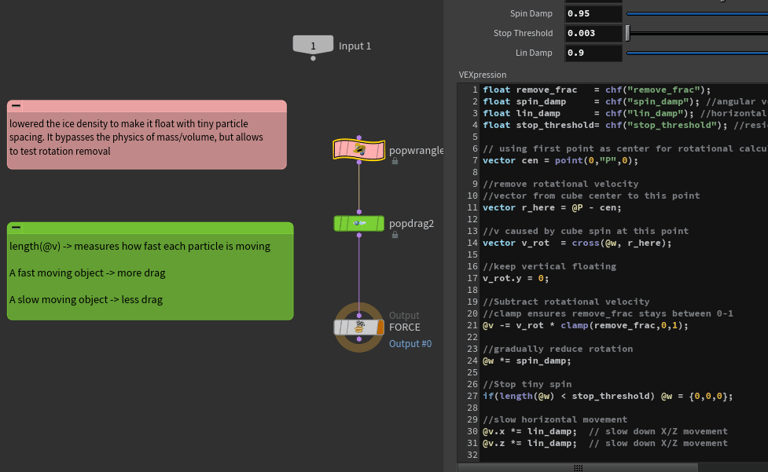
When I set the ice cube’s density to 190, it finally started floating on the surface of the fluid particles. However, an issue arose because the fluid particles hadn’t fully settled, causing the ice cube to continue rotating on the surface. To fix this, I tried a method to slow down the velocity (@v) of the fluid particles, helping them stabilize and reduce unwanted motion.

From the flipbook above, you can see that the particle velocity (@v) slows down a bit, but the ice cube still keeps rotating unnaturally. To fix this, I used the vex above and adjusted the parameter values to achieve a more realistic floating motion.

This approach reduces the ice cube’s unwanted spinning and side-to-side rotating while letting it keep floating naturally.

• remove_frac -> controls how much of the spin velocity gets removed each frame.

• spin_damp -> slowly reduces the angular velocity (@w), like friction against spinning.

• lin_damp -> slows down X/Z movement of the cube.

• stop_threshold -> once the spin is minimal, it stops completely.

• The cross(@w, r_here) part calculates how each point moves due to rotation, so subtracting it removes that spin motion.

• v_rot.y = 0 ensures the cube floats up and down naturally without being forced.

Overall, this code enables the ice cube to float more realistically, gently rocking on the surface rather than spinning endlessly.

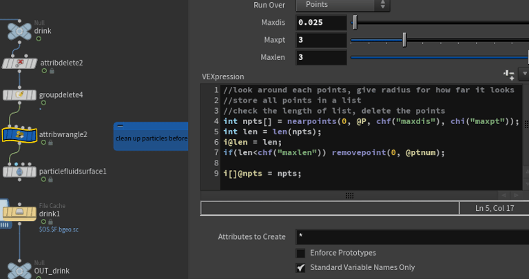
After obtaining a simulation result I liked, I wanted to clean up the particles before converting them into a fluid surface to avoid any strange or messy mesh shapes. I used the following Attribute Wrangle code to remove unnecessary or isolated particles.

• nearpoints(0, @P, chf("maxdis"), chi("maxpt")) -> finds nearby points within a certain distance (maxdis) and limits how many it checks (maxpt).

• len(npts) -> counts how many neighbors each particle has.

• If a particle has fewer neighbors than maxlen, it’s probably isolated or noisy, so it gets deleted with removepoint(0, @ptnum).

The result is a cleaner particle distribution, which makes the Particle Fluid Surface node generate a smoother, more stable mesh.

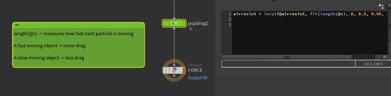
The first thing I tried was using a POP Drag to approach to slow down the particles using this vex above.

I applied this inside the solver because it needs to update every substep to take effect properly.

Explanation:

• length(@v) -> measures the speed of each particle.

• fit(length(@v), 0, 0.5, 0.05, 1.0) -> remaps the particle’s speed from the range 0–0.5 to a new range 0.05–1.0.

• This means slower particles have a smaller air resistance value (0.05), while faster particles have a higher value (1.0).

• lerp(f@airresist, new_value, 0.2) -> smoothly blends between the current air resistance and the new value by 20%.

  This makes the transition smoother instead of changing instantly.

Overall, this setup slows down fast-moving particles more strongly, helping the simulation stabilize gradually rather than stopping too suddenly.

Final ice cube movement

Final mesh

MPM - Setup

Fluid–Soft Body Interaction in MPM Solver

You can combine a soft body and a fluid using the MPM Solver in Houdini by integrating a Gas OpenCL solver and a DOP Network, allowing both materials to simulate within a single system.

Inside a SOP Solver, you can have the soft body (e.g., banana) points check for nearby fluid (e.g., milk) points. When they get close, increase the soft body’s @wet attribute. This attribute can then drive a blend between the source MPM and target MPM using a lerp.

• As @wet increases:

• The soft body’s @E (stiffness) decreases -> becomes softer

• The soft body’s density increases -> becomes heavier

• You can also adjust Critical Compression or Critical Stretch values to allow the soft body to break naturally under stress.

I haven’t tested this yet....i might come back and try after my thesis....... but if you want to try blending a banana or a cookie into a fluid, these are the steps you could follow.

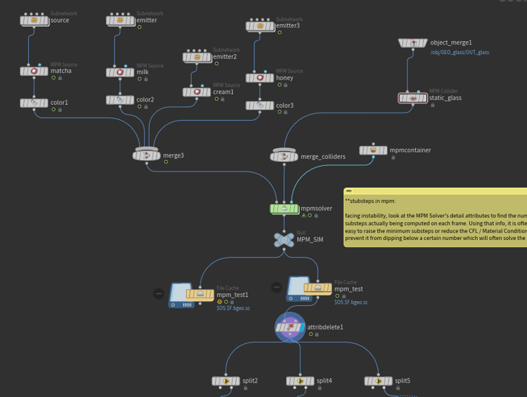
Next, I wanted to use the MPM Solver to simulate four different substances together — matcha, milk, cream, and honey. The MPM method is very efficient because you can feed all these sources into a single MPM Source connected to one solver.

Above is a basic setup for the MPM simulation. One important thing to remember is that MPM is volume-based, so it needs a container to hold the material volume. You must assign this container geometry in the MPM Source node.

In the source, you can easily select from various material types, including fluid, honey, and metal. Each behaves differently.

To achieve the desired color blending of the matcha and milk, I added a @Cd (color) attribute to the source before feeding it into the solver. This allows the colors to mix dynamically during the simulation. (see the steps on the following section)

The MPM Source node also lets you control several key physical parameters, such as density, stiffness, and viscosity, along with other material attributes, depending on the effect you want.

One thing to note about MPM is that it can simulate many different types of materials, so the default substep range is between 1 and 1000.

If you encounter instability in the simulation, check the MPM Solver’s details view to see how many substeps are actually being computed each frame. Based on that information, you can:

• Increase the minimum substeps, or

• Reduce the CFL / Material Condition values

Doing so helps prevent the substeps from dropping too low and usually fixes most stability issues.

computed substeps in solver

Mixing two fluids of different colors

To blend two fluids of different colors in the MPM Solver, I utilized a SOP Solver within DOPs. In the SOP Solver, I brought in the DOP geometry and used an Attribute Transfer node to transfer both @Cd (color) and @density between the two fluid sources.

By adjusting the Max Sample Count and Distance Threshold parameters in the Attribute Transfer node, I was able to control how smoothly the colors and densities blended.

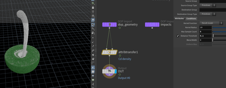
After the simulation is complete, you can use a Split SOP by the name attribute to separate different materials. Then, use Attribute Transfer to transfer the @Cd (color) from the solver back onto the MPM Surface mesh.

icy fractured look insid ice cube

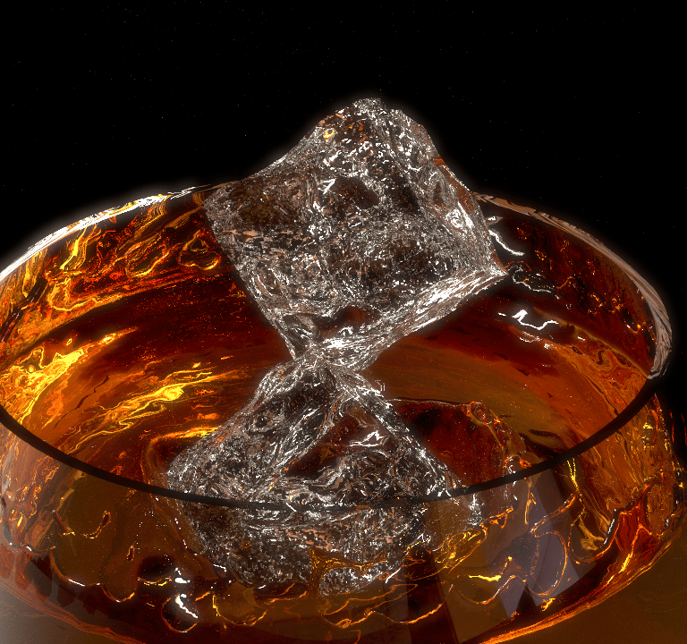
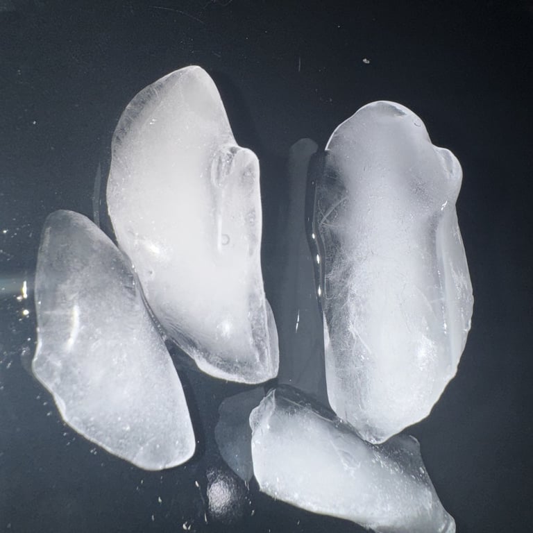
For the ice cube, I aimed to create an icy, fractured look inside. Here’s the workflow I used:

• I created a bounding volume slightly larger than the ice cube, which allows me to use a Boolean operation safely.

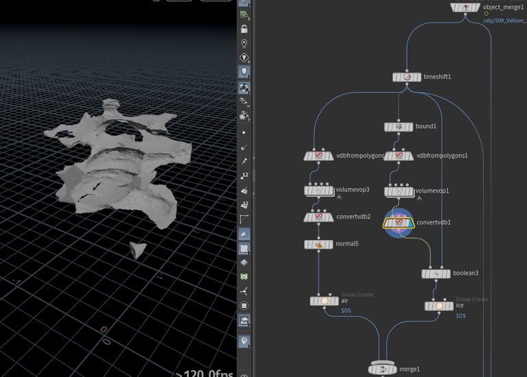
• I converted a polygon version of the cube to a VDB and used a Volume VOP to add noise to the @P positions. This noise drives variations in the density.

• I transferred the modified VDB data back to the polygon and applied a Boolean with the original ice cube to create the fractured look.

• For smaller fracture pieces inside the cube, I used the same process, but without the bounding volume. I converted them, merged them with the main geometry, and then used Point Deform to animate these pieces along with the simulation.

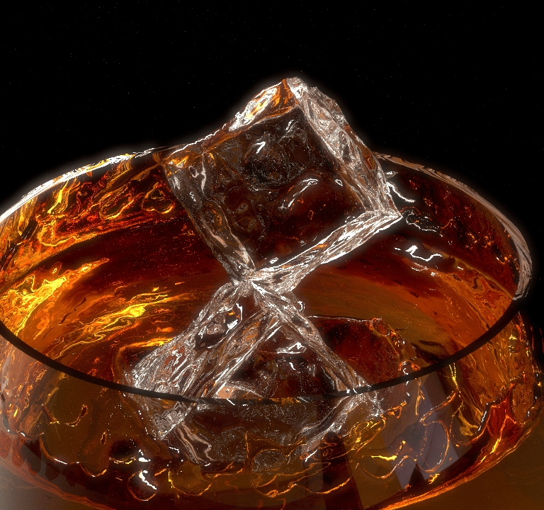
no fracture

fracture